The Horace-SpinW interface

How to use a SpinW model in Horace for fitting

Defining models in Horace: a recap

Horace accepts a variety of functions to model data:

`y = fn(x1, x2, ..., xn, pars)`	Functions operating directly on data coordinates (e.g. gaussian peaks)
`s = fn(qh, qk, ql, en, pars)`	Model $S(\mathbf{q},\omega)$ functions evaluated for each $\omega$
`[w, s] = fn(qh, qk, ql, pars)`	General model $S(\mathbf{q},\omega)$ functions

In all cases, immediately following the coordinates, Horace expects a vector of parameter values to be fitted

After this parameter values, Horace also accepts any other input variables as model constants which will be passed to the model

The fit functions generally only accept the s = fn(qh, qk, ql, en, pars) form for $S(\mathbf{q}, \omega)$ models, so energy convolution needs to be done by the modelling code

The SpinW `spinwave` method: a recap

In order to calculate the spin wave spectrum in SpinW, something like the following needs to be used:


spec = sw_obj.spinwave(hkl, 'hermit', false, 'formfact', true);
spec = sw_egrid(spec, 'component', 'Sperp', 'Evect', 0:0.05:10);

Comparing with what Horace needs, we notice that:

The model (fittable) parameters are not set here, but much earlier in the definition of the model
We need the combination of both spinwave and sw_egrid to get a function of the form s = fn(qh, qk, ql, en, pars) which Horace needs

Fortunately the wrapped model function is provided in SpinW: the method spinw.horace_sqw

The `spinw.horace_sqw` method

horace_sqw has the same signature as a standard Horace $S(\mathbf{q}, \omega)$ function, horace_sqw(qh, qk, ql, en, pars, varargin)

So, it can be used directly in a Horace multifit_sqw call.

In order to define which model parameter is to be varied in the fit, you have to give horace_sqw a mat parameter which is a cell array of the matrix names to be varied in the order they appear in the pars vector

Since the parameters of pars are scalars, if the matrix you refer to is not isotropic (e.g. it's not representing a Heisenberg interaction), a special syntax to refer to which matrix element(s) needs to vary has to be used.

A simple example:


J = 1.2;
K = 0.1;
tri = sw_model('triAF', J);
tri.addmatrix('label', 'K', 'value', diag([0 0 K]));
tri.addaniso('K');

fwhm = 0.75;
scalefactor = 1;
ws = cut_sqw(sqw_file, [0.05], [-0.1, 0.1], [-0.1, 0.1], [0.5]);
fitobj = multifit_sqw(ws);
fitobj.set_fun(@tri.horace_sqw);
fitobj.set_pin({[J K fwhm scalefactor], 'mat', {'J_1', 'K(3,3)'}, ...
    'hermit', false, 'useFast', true, 'formfact', true});
ws_sim = fitobj.simulate();
[ws_fit, fit_dat] = fitobj.fit()

The vector [J K fwhm scalefactor] is the parameters vector. We need to tell SpinW that it corresponds to the Heisenberg nearest neighbour interaction J_1 and the easy-place anisotropy K

Because J is isotropic, we can just give the matrix name in mat

But, K only applies to the zz element, so we need to tell SpinW that in mat

fwhm and scalefactor are parameters which are added by horace_sqw to denote the energy FWHM and intensity scale factor (may be omitted, in which case it is taken to be unity and fixed)

The other (non-varying) parameters we pass to multifit are just standard SpinW keyword arguments

There are a few keyword arguments unique to horace_sqw

'useFast' - This tells horace_sqw to use a faster but slightly less accurate code than spinwave. In particular, this code achieves a speed gain by:

Only calculating Sperp rather than full $S^{\alpha\beta}$ tensor
Only calculating magnon creation (positive energy / neutron energy loss) modes.
Ignoring twins

'partrans' - A function handle to transform the input parameters received from Horace before passing to SpinW
'coordtrans' - A $4\times 4$ matrix to transform the input $(Q_h, Q_k, Q_l, \hbar\omega)$ coordinates received from Horace before passing to SpinW
'resfun' - This is tells horace_sqw what function to use for the energy convolution. Options are:

'gauss' - a gaussian (one parameter: fwhm)
'lor' - a lorentzian (one parameter: fwhm)
'voigt' - a pseudovoigt (two parameters: fwhm and lorentzian fraction)
'sho' - a damped harmonic oscilator (parameters: Gamma Temperature Amplitude)
A function handle to a function which will be accepted by Horace's disp2sqw method

horace_sqw appends the parameters needed by resfun to the end of the parameter vector and then adds a scale factor between the data and calculation after that

The `'mat'` argument

Horace expects a parameter vector, so we have to tell SpinW which parameter is which

In simple cases, just the name of the corresponding SpinW matrix, or a string denoting which single matrix element suffice

For more complicated cases, an additional parameter 'selector', a $3\times3$ logical matrix needs to be used

This tells the matparser function which SpinW uses to decode the 'mat' argument which matrix elements the parameter corresponds to

Dvec = [0.1 0.2 0.3];
swobj.addmatrix('label', 'DM', 'value', Dvec);
swobj.addcoupling('mat', 'DM', 'bond', 1);

sel(:,:,1) = [0 0 0; 0 0 1; 0 -1 0];    % Dx
sel(:,:,2) = [0 0 1; 0 0 0; -1 0 0];    % Dy
sel(:,:,3) = [0 1 0; -1 0 0; 0 0 0];    % Dz

fitobj.set_fun(@swobj.horace_sqw);
fitobj.set_pin({Dvec, 'mat', {'DM', 'DM', 'DM'}, ...
    'selector', sel, 'hermit', false})
fitobj.fit()

'selector' is a $3\times 3\times N$ array where $N$ is the number of parameters

Each $3\times 3$ matrix denotes which elements of the corresponding matrix in 'mat' goes with that parameter

Mex files in SpinW

How to speed up your calculations with parallelised compiled helper libraries

SpinW mex files

SpinW contains a few C libraries to speed up the spin wave calculations

They perform standard linear algebra algorithms on stacks of matrices in parallel.

`eig_omp`	Calculates eigenvalues / eigenvectors of a stack of matrices
`chol_omp`	Calculates the Cholesky factorisation of a stack of matrices
`sw_mtimesx`	Calculates matrix-matrix or matrix-vector multiplications

For each $\mathbf{q}$ SpinW has to diagonalise or solve a Hamiltonian matrix. If this could be done in parallel there will be a speed up (typically around 2-3 times for a 4-core computer).

The 'optmem' option in spinwave determines how many $\mathbf{q}$'s are calculated at once - the more $\mathbf{q}$'s, the greater the speed up (hence more memory is better!)

Using mex files in SpinW

To tell SpinW to use the mex'ed libraries, do:


swpref.setpref('usemex',true)

You can just type swpref again to show all the options

If the distributed compiled mex files are not compatible with your system you will get an error

Compiling SpinW mex files

The SpinW distribution contains compiled versions of these files for the standard 64-bit operating systems (Windows, Linux and Mac OS X), but in case you need to compile it yourself...

First, to compile the mex files, you will need to have installed a Matlab-compatible compiler - see: https://uk.mathworks.com/support/compilers.html

This is generally Visual Studio in Windows, gcc on Linux and XCode on Mac.

(Note that on Mac OS X you will need to use homebrew as OpenMP is not supported by the standard XCode compiler)

Set up mex using:


mex -setup

Then compile the SpinW mex files with:


sw_mex

Or:


sw_mex('test', true)

To run a test suite which will also tell you how much of a speed up you might expect (it takes ~5min to run).

Example of Horace-SpinW integration

Modelling spin waves in Pr(Ca_0.9Sr_0.1)₂Mn₂O₇
Download the scripts here: pcsmo_eval.m

Published data and simulation of Pr(Ca$_{0.9}$Sr$_{0.1}$)$_2$Mn$_2$O$_7$

Pr(Ca_0.9Sr_0.1)₂Mn₂O_{7 Horace data}

The .sqw files should be in the folders previously used for Horace

If you're not using a desktop, you can get the files from: Dropbox

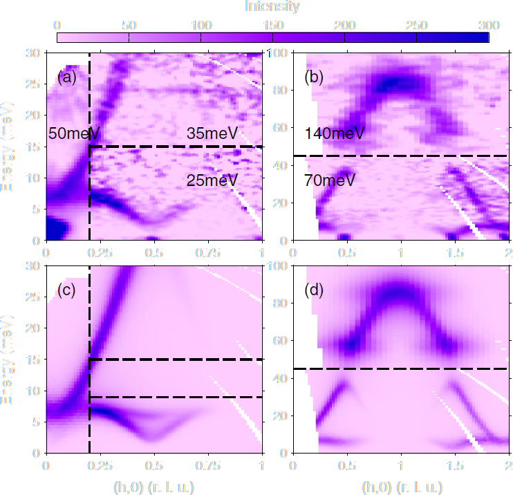
Make 2D slices along $(h00)$ and energy transfer and compare to figure 2 of Johnstone et al.


ei = [25 35 50 70 140];
proj = projaxes([1 0 0], [0 1 0]);
for ii = 1:numel(ei);
    sqw_file = sprintf('../aaa_my_work/pcsmo_ei%d_base.sqw', ei(ii));
    ws_cut(ii) = cut_sqw(sqw_file, proj, [-5,0.025,5], [-0.2,0.2], ...
        [-inf,inf], [ei(ii)/100]);
    % Symmetrise about h=0
    ws_cut(ii) = symmetrise_sqw(ws_cut(ii), [0 0 1], [0 1 0], [0 0 0]);
    plot(ws_cut(ii))
    lz 0 10
    keep_figure;
end

Background subtraction

As in the Horace tutorials, make a cut at high $q$ and use replicate to generate a 2D background slice

Subtract this from the data and compare it to the paper


for ii = 1:numel(ei)
    idx = find(sum(ws_cut(ii).data.s,2)>0);
    qmax = ws_cut(ii).data.p{1}(idx(end)) * 0.5;
    ws_bkg(ii) = cut_sqw(ws_cut(ii), [qmax-0.1,qmax], []);
    ws_sub(ii) = ws_cut(ii) - replicate(ws_bkg(ii), ws_cut(ii));
    plot(ws_sub(ii))
    lz 0 10
    lx -2 2
    keep_figure; 
end

Evaluate the SpinW model

Use the code from the previous ("real world") tutorial to set up a SpinW model of the Goodenough model

Evaluate this model on the cuts you've made:

Because the model had to use a larger ($2\times 2\times 1$) "structural" unit cell, we need to convert the $Q_h$ and $Q_k$ coordinates given by Horace (multiply them by 2) to get the SpinW equivalent:


cpars = {'coordtrans', diag([2 2 1 1])}

Add the usual SpinW options:


cpars = {cpars{:}, 'mat', {'JF1', 'JA', 'JF2', 'JF3', 'Jperp', 'D(3,3)'}, ...
    'hermit', false, 'optmem', 0, 'useFast', true, 'formfact', true, ...
    'resfun', 'gauss'};

Select the 170 meV dataset to see the overal dispersion (including gap)

Then set up a multifit object on this dataset - use a dnd object to save time (the sqw object will have ~100x the number of pixels)

Finally tell SpinW to use mex files to speed up the calculation and evaluate the SpinW model


idx = 5;            % EIs: [25 35 50 70 140], index 5 == 140meV 
fwhm = ei(idx)/30;  % Typical resolution ~ 3% of Ei  

kk = multifit_sqw(d2d(ws_sub(idx)));
kk = kk.set_fun (@pcsmo.horace_sqw, {[JF1 JA JF2 JF3 Jperp D fwhm] cpars{:}}); 
kk = kk.set_free ([1, 1, 1, 1, 1, 1, 1]); 
kk = kk.set_options ('list',2);  

swpref.setpref('usemex',true);  
% Time a single iteration 
tic 
wsim = kk.simulate; 
t_spinw_single = toc;

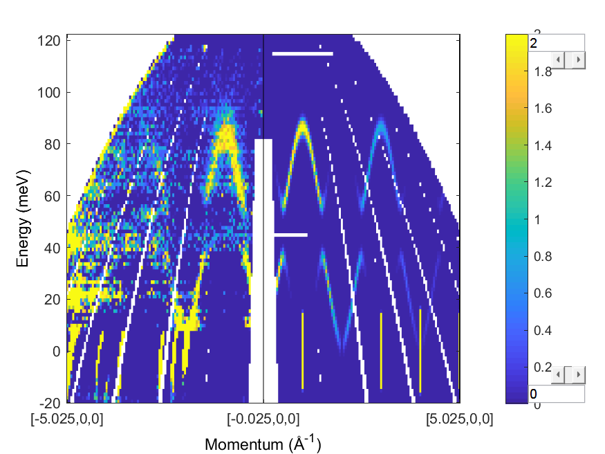
Published data and SpinW simulation of Pr(Ca$_{0.9}$Sr$_{0.1}$)$_2$Mn$_2$O$_7$

Plot the simulation

Reflect the data back to the negative $Q_h$ side, remove the empty bins (with compact )

Convert the data to a d2d object and then use spaghetti_plot to plot the data and simulation (already a d2d object) together


wss = symmetrise_sqw(ws_sub(idx),[0 1 0],[0 0 1],[0 0 0]);
spaghetti_plot([compact(d2d(wss)) compact(wsim)])
lz 0 2

Example of Horace-SpinW fitting

Fitting spin waves in bcc-Iron with SpinW and Horace
Download the scripts here: fe_fit.m

Make the set of standard $Q_h$ 1D cuts at different energies as before


proj = projaxes([1 1 0], [-1 1 0]);
energy_range = [80:20:160];
for i = 1:numel(energy_range)
    my_cuts(i) = cut_sqw(sqw_file, proj, [-3,0.05,3], [-1.05,-0.95], [-0.05,0.05], ...
        [-10 10]+energy_range(i)); 
end

Run the same fits with the analytical $S(\mathbf{q},\omega)$ function as before and note the fitted parameters and how long it takes

Define a SpinW model for bcc-Fe with a single nearest neighbour exchange and a small easy axis anisotropy


a = 2.87;

fe = spinw;
fe.genlattice('lat_const', [a a a], 'angled', [90 90 90], 'spgr', 'I m -3 m')  % bcc Fe
fe.addatom('label', 'MFe3', 'r', [0 0 0], 'S', 5/2, 'color', 'gold')
fe.gencoupling()
fe.addmatrix('label', 'J1', 'value', 1, 'color', 'gray')
fe.addmatrix('label', 'D', 'value', diag([0 0 -1]), 'color', 'green')
fe.addcoupling('mat', 'J1', 'bond', 1)
fe.addaniso('D')
fe.genmagstr('mode', 'direct', 'S', [0 0 1; 0 0 1]');  % Ferromagnetic

plot(fe, 'range', [2 2 2])

Set the parameters for the fits, and also SpinW options

Note that the analytical expression used previous for $S(\mathbf{q},\omega)$ used $JS$, whereas SpinW uses $J$, and we have defined $S=\frac{5}{2}$


% Initial parameters:
J = -16;
D = -0.1;
gam = 66;
temp = 10;
amp = 131;

cpars = {'mat', {'J1', 'D(3,3)'}, 'hermit', false, 'optmem', 1, ...
    'useFast', true, 'resfun', 'sho', 'formfact', true}; 
swpref.setpref('usemex',true);

Notice that we use the sho resolution function, in common with the analytical expressions

Because the cuts are small, we also force SpinW to calculate all q-points in one chunk with the {'optmem', 1} option.

Set up the multifit object on the array of 1D cuts

Use the horace_sqw method as the fit function and parameters as defined previously, and run the fit


kk = multifit_sqw (my_cuts);
kk = kk.set_fun (@fe.horace_sqw, {[J D gam temp amp] cpars{:}});
kk = kk.set_free ([1, 0, 1, 0, 1]);
kk = kk.set_bfun (@linear_bg, [0.1,0]);
kk = kk.set_bfree ([1,0]);
kk = kk.set_options ('list',2);

[wfit, fitdata] = kk.fit('comp');

Compare the fits - are the parameters or correlation matrix consistent?

SpinW and Horace