spinw.powspec method

Syntax

spectra = powspec(obj,QA)

spectra = powspec(___,Name,Value)

Description

spectra = powspec(obj,QA) calculates powder averaged spin wave spectrum by averaging over spheres with different radius around origin in reciprocal space. This way the spin wave spectrum of polycrystalline samples can be calculated. This method is not efficient for low dimensional (2D, 1D) magnetic lattices. To speed up the calculation with mex files use the swpref.setpref('usemex',true) option.

spectra = powspec(___,Value,Name) specifies additional parameters for the calculation. For example the function can calculate powder average of arbitrary spectral function, if it is specified using the specfun option.

Example

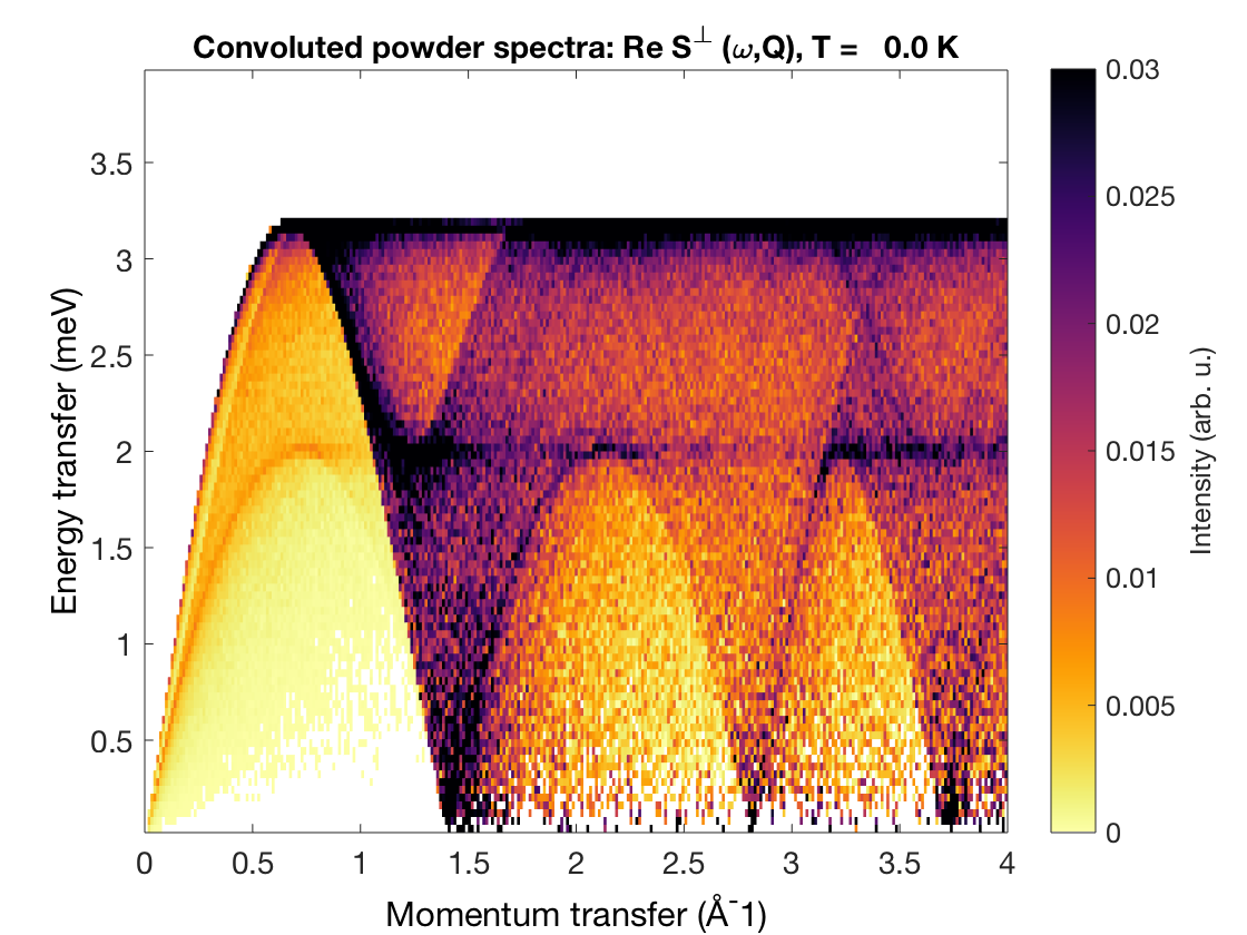
Using only a few lines of code one can calculate the powder spectrum of the triangular lattice antiferromagnet (\(S=1\), \(J=1\)) between \(Q=0\) and 3 Å\(^{-1}\) (the lattice parameter is 3 Å).

tri = sw_model('triAF',1);
E = linspace(0,4,100);
Q = linspace(0,4,300);
triSpec = tri.powspec(Q,'Evect',E,'nRand',1e3);
sw_plotspec(triSpec);

Input arguments

obj: spinw object.
QA: Vector containing the \(Q\) values in units of the inverse of the length unit (see spinw.unit) with default unit being Å\(^{-1}\). The value are stored in a row vector with \(n_Q\) elements.

Name-Value Pair Arguments

specfun

Function handle of a solver. Default value is @spinwave. It is currently tested with two functions:

spinw.spinwave Powder average spin wave spectrum.
spinw.scga Powder averaged diffuse scattering spectrum.

nRand

Number of random orientations per QA value, default value is 100.

Evect

Row vector, defines the center/edge of the energy bins of the calculated output, number of elements is \(n_E\). The energy units are defined by the spinw.unit.kB property. Default value is an edge bin linspace(0,1.1,101).

binType

String, determines the type of bin, possible options:

'cbin' Center bin, the center of each energy bin is given.
'ebin' Edge bin, the edges of each bin is given.

Default value is 'ebin'.

'T'

Temperature to calculate the Bose factor in units depending on the Boltzmann constant. Default value taken from obj.single_ion.T value.

'title'

Gives a title to the output of the simulation.

'extrap'

If true, arbitrary additional parameters are passed over to the spectrum calculation function.

'fibo'

If true, instead of random sampling of the unit sphere the Fibonacci numerical integration is implemented as described in J. Phys. A: Math. Gen. 37 (2004) 11591. The number of points on the sphere is given by the largest Fibonacci number below nRand. Default value is false.

'imagChk'

Checks that the imaginary part of the spin wave dispersion is smaller than the energy bin size. Default value is true.

'component'

See sw_egrid for the description of this parameter.

The function also accepts all parameters of spinw.spinwave with the most important parameters are:

'formfact'

If true, the magnetic form factor is included in the spin-spin correlation function calculation. The form factor coefficients are stored in obj.unit_cell.ff(1,:,atomIndex). Default value is false.

'formfactfun'

Function that calculates the magnetic form factor for given \(Q\) value. value. Default value is @sw_mff, that uses a tabulated coefficients for the form factor calculation. For anisotropic form factors a user defined function can be written that has the following header:

F = formfactfun(atomLabel,Q)

where the parameters are:

F row vector containing the form factor for every input \(Q\) value
atomLabel string, label of the selected magnetic atom
Q matrix with dimensions of \([3\times n_Q]\), where each column contains a \(Q\) vector in \(Å^{-1}\) units.

'gtensor'

If true, the g-tensor will be included in the spin-spin correlation function. Including anisotropic g-tensor or different g-tensor for different ions is only possible here. Including a simple isotropic g-tensor is possible afterwards using the sw_instrument function.

'hermit'

Method for matrix diagonalization with the following logical values:

true using Colpa’s method (for details see J.H.P. Colpa, Physica 93A (1978) 327), the dynamical matrix is converted into another Hermitian matrix, that will give the real eigenvalues.
false using the standard method (for details see R.M. White, PR 139 (1965) A450) the non-Hermitian \(\mathcal{g}\times \mathcal{H}\) matrix will be diagonalised, which is computationally less efficient. Default value is true.

Note: Always use Colpa’s method, except when imaginary eigenvalues are expected. In this case only White’s method work. The solution in this case is wrong, however by examining the eigenvalues it can give a hint where the problem is.

'fid'

Defines whether to provide text output. The default value is determined by the fid preference stored in swpref. The possible values are:

0 No text output is generated.
1 Text output in the MATLAB Command Window.
fid File ID provided by the fopen command, the output is written into the opened file stream.

'tid'

Determines if the elapsed and required time for the calculation is displayed. The default value is determined by the tid preference stored in swpref. The following values are allowed (for more details see sw_timeit):

0 No timing is executed.
1 Display the timing in the Command Window.
2 Show the timing in a separat pup-up window.

The function accepts some parameters of [spinw.scga] with the most important parameters are:

'nInt': Number of \(Q\) points where the Brillouin zone is sampled for the integration.

Output Arguments

spectra

structure with the following fields: