Syntax
p = sw_res(source,poldeg)
p = sw_res(source,poldeg,true)
Description
p = sw_res(fid,poldeg) reads tabulated resolution data from the
source file which contains the FWHM energy resolution values as a
function of energy transfer in two columns. First column is the energy
transfer values (positive is energy loss), while the second is the FWHM
of the Gaussian resolution at the given energy transfer.
p = sw_res(fid,poldeg,plot) the polynomial fit will be shown in a
figure if plot is true.
Examples
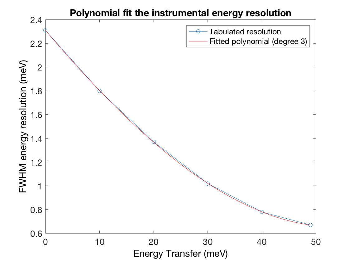
This example shows how to fit a tabulated resolution data (MERLIN energy resolution for \(E_i=50\) meV and 300 Hz chopper frequency). Using the fitted polynomial, the energy resolution can be calculated at an arbitrary energy transfer value.
resDat = [0 2.31;10 1.80;20 1.37;30 1.02;40 0.78;49 0.67]
Output
resDat =
         0    2.3100
   10.0000    1.8000
   20.0000    1.3700
   30.0000    1.0200
   40.0000    0.7800
   49.0000    0.6700
polyRes = sw_res(resDat,3)
EN = 13
dE = polyval(polyRes,EN)
Output
dE =
    1.6635
Input Arguments
source- String, path to the resolution file or a matrix with two columns, where the first column gives the energy transfer value and second column gives the resolution FWHM.
polDeg- Degree of the fitted polynomial, default value is 5.
plot- If
truethe resolution will be plotted, default value istrue.
Output Arguments
p- The coefficients for a polynomial \(p(x)\) of degree \(n\) that is a best fit (in a least-squares sense) for the resolution data. The coefficients in \(p\) are in descending powers, and the length of \(p\) is \(n+1\): \[p(x)=p_1\cdot x^n+p_2\cdot x^{n-1}+...+p_n\cdot x+p_{n+1}\]
See Also
[polyfit] | sw_instrument