Energy cuts and Horace integration

This example shows how to calculate the spin wave spectrum of the square lattice Heisenberg antiferromagnet and to produce a constant energy cut of the spectrum.

Contents

Crystal & magnetic structure

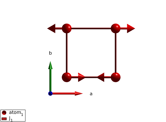
Using sw_model, the crystal and magnetic structure are readily available. Using the 'squareAF' option, a square lattice Heisenberg Antiferromagnet with S = 1 and J = 1 is created.

sq = sw_model('squareAF',1,0);

% We add magnetic form factor after the model is defined. Using the same
% atom label and position as an existing atom in the model, the atom
% properties will be updated, no new atom is created using the
% spinw.addatom method. We will use the form factor of Ni2+ that has S=1.

sq.addatom('label','atom_1','r',[0 0 0],'formfact','MNi2+','S',1)
plot(sq)
swplot.zoom(2)

Warning: The x-ray scattering form factor for atom_1+ is undefined, constant 1
will be used instead! If you don't want to see this message add a line to
xrayion.dat (use the 'edit xrayion.dat' command) for the corresponding ion! 
Warning: The neutron scattering length for atom_1 is undefined, constant 1 will
be used instead! 

Spin wave

We need to define a grid in reciprocal space, here we use the (Qh, Qk, 0) square lattice plane by calling ndgrid() function.

nQ = 201;
nE = 501;
Qhv = linspace(0,2,nQ);
Qkv = linspace(0,2,nQ);
Qlv = 0;
[Qh, Qk, Ql] = ndgrid(Qhv,Qkv,Qlv);

% Create a list of Q point, with dimensions of [3 nQ^2].
Q = [Qh(:) Qk(:) Ql(:)]';

Spin wave spectrum

We calculates the spin wave spectrum at the list of Q points, bin the diagonal of the spin-spin correlation function (Sxx+Syy+Szz) in energy and convolute with a finite instrumental resolution.

spec = sq.spinwave(Q);

Ev = linspace(0,5,nE);
spec = sw_egrid(spec,'component','Sxx+Syy+Szz','Evect',Ev);
spec = sw_instrument(spec,'dE',0.1);

Creat the Q map

The calculated intensity map is stored in spec.swConv, we reshape it into a 3D matrix using Matlab commands.

spec3D = reshape(spec.swConv,nE-1,nQ,nQ);

Plotting E=const cut

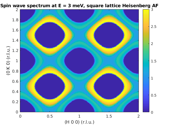
A constant energy cut takes the (Eidx,:,:) elements of the matrix and plots it using the Matlab function imagesc(). We also integrate in energy the same way Horace does by taking the average of the points and rescaling with the energy bin size.

Ecut = [3.5 4.0]; %meV
Eidx = find(Ev>Ecut(1) & Ev<Ecut(2));
figure;
cut1 = squeeze(sum(spec3D(Eidx,:,:),1))/numel(Eidx)/(Ev(2)-Ev(1));
imagesc(Qhv,Qkv,cut1);
set(gca,'YDir','normal')
xlabel('(H 0 0) (r.l.u.)')
ylabel('(0 K 0) (r.l.u.)')
title('Spin wave spectrum at E = 3 meV, square lattice Heisenberg AF')
caxis([0 3])
colorbar

Constant energy cut using Horace

We can do the same cut much easyer using Horace (http://horace.isis.rl.ac.uk). Assuming that Horace is installed and initialized we can do the same constant energy cut with just three steps. First we create an empty d3d object that defines the (h,k,0) plane with ranges in momentum and energy. Second we call Horace to fill up the empty d3d object with the simulated spin wave data and finally we plot a constant energy cut.

if ~exist('sqw','file')
    fprintf('Horace is not installed. Exiting....\n');
    return
end

Ebin   = [0,0.01,5];
fwhm0  = 0.1;
d3dobj = d3d(sq.abc,[1 0 0 0],[0,0.01,2],[0 1 0 0],[0,0.01,2],[0 0 0 1],Ebin);
d3dobj = disp2sqw_eval(d3dobj,@sq.horace,{'component','Sxx+Syy+Szz'},fwhm0);
plot(cut(d3dobj,[],[],[3.5 4]));
colorslider('delete')
title('')
caxis([0 3])
colorbar

Horace is not installed. Exiting....

Spaghetti plot using Horace

Horace can be also used to generate cuts along certain line in the Brillouin zone. The advantage of this approach is that it can be better combined with data treatment in Horace. Where the sample plot can be calculated on real pixel data using the spaghetti_plot function.

Qlist  = [0 0 0;0 1/2 0;1/2 1/2 0;0 0 0];
Qlabel = {'\Gamma' 'X' 'M' '\Gamma'};
Ebin   = [0 0.01 5];
fwhm0  = 0.1;

disp2sqw_plot(Qlist,@sq.horace,{},Ebin,fwhm0,'labels',Qlabel)
colorslider('delete')
caxis([0 3])
colormap(flipud(cm_inferno))
colorbar

Written by
Sandor Toth
06-Jun-2014, 08-Feb-2017

Published with MATLAB® R2018b