Antiferromagnetic nearest-neighbour spin chain

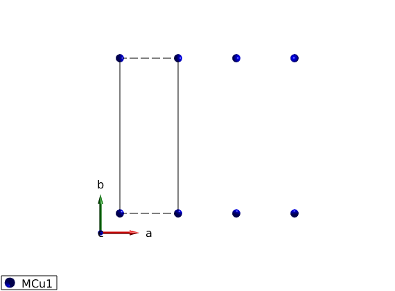
Definition of crystal structure, shortest bonds along the a-axis magnetic Cu+ atoms with S=1 spin.

Contents

Define the lattice

AFMchain = spinw;
AFMchain.genlattice('lat_const',[3 8 8],'angled',[90 90 90],'spgr',0);
AFMchain.addatom('r',[0 0 0],'S',1,'label','MCu1','color','blue');
disp('Magnetic lattice:')
AFMchain.table('matom')
plot(AFMchain,'range',[3 1 1])

Magnetic lattice:

ans =

  1×4 table

    matom     idx    S        pos    
    ______    ___    _    ___________

    'MCu1'     1     1    0    0    0

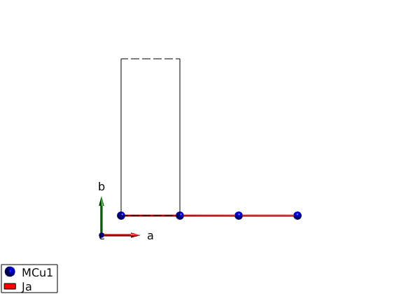
Create antiferromagnetic interactions

Ja = 1 meV, positive sign denotes antiferromagnetic interaction.

AFMchain.gencoupling('maxDistance',7)
AFMchain.table('bond',[1 2])

AFMchain.addmatrix('label','Ja','value',1,'color','red');
AFMchain.addcoupling('mat','Ja','bond',1);
disp('After assigning a matrix to a bond:')
AFMchain.table('bond',[1 2])
plot(AFMchain,'range',[3 0.9 0.9])

ans =

  2×10 table

    idx    subidx        dl             dr         length    matom1    idx1    matom2    idx2        matrix    
    ___    ______    ___________    ___________    ______    ______    ____    ______    ____    ______________

     1       1       1    0    0    1    0    0      3       'MCu1'     1      'MCu1'     1      ''    ''    ''
     2       1       2    0    0    2    0    0      6       'MCu1'     1      'MCu1'     1      ''    ''    ''

After assigning a matrix to a bond:

ans =

  2×10 table

    idx    subidx        dl             dr         length    matom1    idx1    matom2    idx2         matrix     
    ___    ______    ___________    ___________    ______    ______    ____    ______    ____    ________________

     1       1       1    0    0    1    0    0      3       'MCu1'     1      'MCu1'     1      'Ja'    ''    ''
     2       1       2    0    0    2    0    0      6       'MCu1'     1      'MCu1'     1      ''      ''    ''

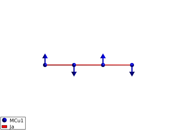
Two ways of defining the magnetic structure

Define all spins

We define a magnetic supercell 2x1x1 of the crystal cell and define both spin direction in the supercell with the following parameters:

AFMchain.genmagstr('mode','direct','k',[1/2 0 0],'n',[1 0 0],'S',[0 0; 1 -1;0 0],'nExt',[2 1 1]);

Define only one spin

We define the spin direction in the crystallographic unit cell and let the sw.genmagstr() function generate the other spin based on the magnetic ordering wave vector and normal vectors. This method is usefull for creating complex structures. Both methods gives the same magnetic structure, all stored values in the afchain.mag_str field are the same.

AFMchain.genmagstr('mode','helical','k',[1/2 0 0],'n',[1 0 0],'S',[0; 1; 0],'nExt',[2 1 1]);
disp('Magnetic structure:')
AFMchain.table('mag')

% Ground state energy
AFMchain.energy
plot(AFMchain,'range',[3 0.9 0.9],'cellMode','none','baseMode','none')

Magnetic structure:

ans =

  2×8 table

    num    matom     idx    S      realFhat         imagFhat           pos              kvect      
    ___    ______    ___    _    _____________    _____________    ___________    _________________

     1     'MCu1'     1     1    0     1     0    0     0     1    0    0    0    0.5      0      0
     2     'MCu1'     1     1    0    -1     0    0     0    -1    1    0    0    0.5      0      0

Ground state energy: -1.000 meV/spin.

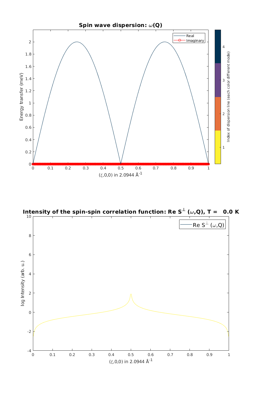
Spin wave spectrum

We calculate the spin wave spectrum and neutron scattering cross sections along the chain direction. The neutron scattering cross section is plotted together with the dispersion (black line).

afcSpec = AFMchain.spinwave({[0 0 0] [1 0 0] 523}, 'hermit',true);
figure
subplot(2,1,1)
sw_plotspec(afcSpec,'mode',4,'dE',0.2,'axLim',[0 3])

% To calculate the intensity, we need to sum up the intensity of the two
% degenerate spin wave mode using the sw_omegasum() function. We plot the
% logarithm of the intensity.

afcSpec = sw_neutron(afcSpec);
afcSpec = sw_egrid(afcSpec,'Evect',linspace(0,6.5,500),'component','Sperp');
afcSpec = sw_omegasum(afcSpec,'zeroint',1e-6);
subplot(2,1,2)
sw_plotspec(afcSpec,'mode',2,'log',true,'axLim',[-4 10])

% Position the figure on the screen, similarly how subplot() positions the
% axes on the figure.
swplot.subfigure(1,3,1)

Written by
Bjorn Fak & Sandor Toth
06-Jun-2014, 06-Feb-2015

Published with MATLAB® R2018b