Spin wave disperion of YVO3

We compare our results with the model from: C. Ulrich, et al. PRL 91, 257202 (2003). see [[http://prl.aps.org/abstract/PRL/v91/i25/e257202]] We create crystal structure of YVO3 in the pseudocubic unit cell, doubled along c-axis. The magnetic atoms are V4+ with spin quantum number S=1/2.

Contents

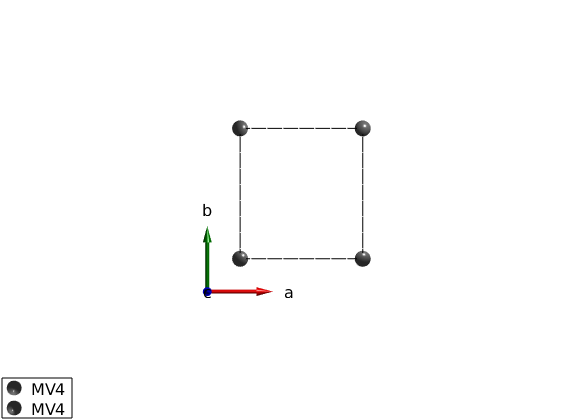
Define the lattice

a = 5.2821;
b = 5.6144;
c = 7.5283;

yvo3 = spinw;
yvo3.genlattice('lat_const', [a/sqrt(2) b/sqrt(2) c]);
yvo3.addatom('r',[0 0 0],'label','MV4','S',1/2,'color','gray')
yvo3.addatom('r',[0 0 1/2],'label','MV4','S',1/2,'color','gray')
yvo3.gencoupling
%yvo3.newcell({[1 1 0] [-1 1 0] [0 0 1]})
plot(yvo3)

Warning: The x-ray scattering form factor for V4+ is undefined, constant 1 will
be used instead! If you don't want to see this message add a line to xrayion.dat
(use the 'edit xrayion.dat' command) for the corresponding ion! 
Warning: The x-ray scattering form factor for V4+ is undefined, constant 1 will
be used instead! If you don't want to see this message add a line to xrayion.dat
(use the 'edit xrayion.dat' command) for the corresponding ion! 

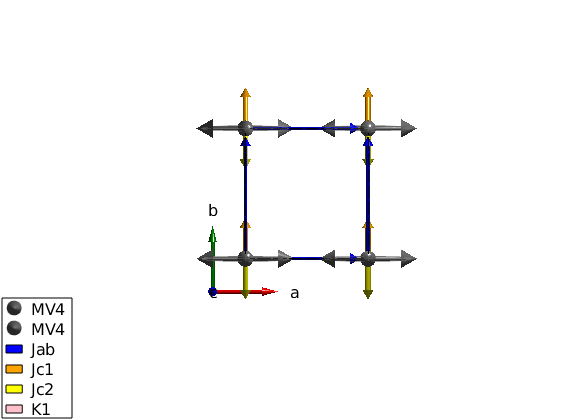
Magnetic Hamiltonian

The exchange constants are taken from the paper.

Jab   = 2.6;
Jc    = 3.1;
delta = 0.35;
K1    = 0.90;
K2    = 0.97;
d     = 1.15;

%Calculate the canting angle in the ac-plane:
theta = 1/2*atan(2*d/(2*Jc-K1-K2));
%Define matrices for the Hamiltonian:

Jc1 = -Jc*(1+delta)*eye(3) + diag([K2 0 0]) - [0 0 d;0 0 0;-d 0 0];
Jc2 = -Jc*(1-delta)*eye(3) + diag([K2 0 0]) + [0 0 d;0 0 0;-d 0 0];

yvo3.addmatrix('label','Jab','value',Jab,'color','blue')
yvo3.addmatrix('label','Jc1','value',Jc1,'color','orange')
yvo3.addmatrix('label','Jc2','value',Jc2,'color','yellow')
yvo3.addmatrix('label','K1','value',diag([-K1 0 0]),'color','pink')

% Assign the matrices to the magnetic atoms:
yvo3.addcoupling('mat','Jab','bond',[1 3])
yvo3.addcoupling('mat','Jc1','bond',2,'subidx',2)
yvo3.addcoupling('mat','Jc2','bond',2,'subidx',1)

% Add K1 matrix to the single-ion anisotropy:
yvo3.addaniso('K1')

% Create test magnetic structure, G-type antiferromagnet:
par_ms.mode = 'helical';
par_ms.S    = [1;0;0];
par_ms.nExt = [2 2 1];
par_ms.k    = [1/2 1/2 1];
par_ms.n    = [0 1 0];

yvo3.genmagstr(par_ms);

%Plotting magnetic structure with anisotropy ellipsoids:
plot(yvo3)

% Optimising magnetic structure using contrained optimization. Using the
% gm_planard() contrained function, we restrict the solution to planar
% magnetic structures. The meaning of the x parameters are the following:
% (phi1, phi2, ... phiN, kx, ky kz, nTheta, nPhi), where all parameters
% except the propagtion vector are in degree.

par_opt.xmin = [zeros(1,8)   , 0 0 0,   0   0];
par_opt.xmax = [ones(1,8)*360, 0 0 0, 180 180];
par_opt.func = @gm_planar;
par_opt.nRun = 10;

optRes = yvo3.optmagstr(par_opt);
E1 = yvo3.energy;

% To check whether we found the optimum, let's run the unconstrained local
% optimization, spinw.optmagsteep and see if we can reach lower energy.
yvo3.optmagsteep('nRun',1e4);
E2 = yvo3.energy;
dE = E2-E1
nE = 1e3;

% The unconstrained local optimization reached lower energy. Showing that
% it is always good to recheck the results.

dE =

  -8.3446e-09

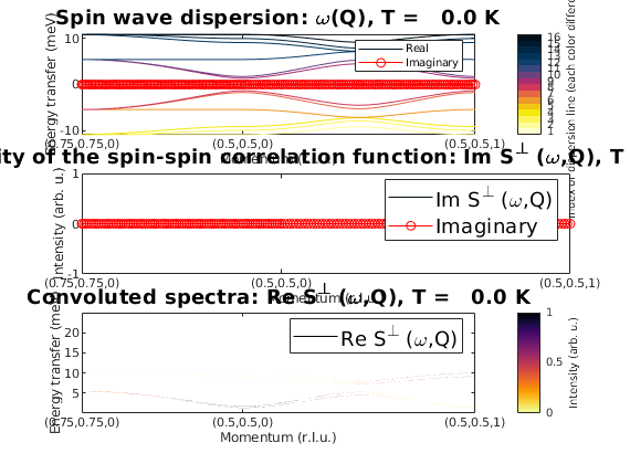
Check canting angles

M   = yvo3.magstr.S;
phi = atan2(M(1,:),M(3,:))*180/pi;

%Calculating spin wave dispersion:
specYVO3 = yvo3.spinwave({[3/4 3/4 0] [1/2 1/2 0] [1/2 1/2 1] });
specYVO3 = sw_neutron(specYVO3);
specYVO3 = sw_egrid(specYVO3,'Evect',linspace(0,25,nE));
%Plotting of spin wave spectra with imaginary components:
figure
subplot(3,1,1);
sw_plotspec(specYVO3,'mode',1,'aHandle',gca,'imag',true);
subplot(3,1,2);
sw_plotspec(specYVO3,'mode',2,'aHandle',gca,'imag',true);
subplot(3,1,3);
sw_plotspec(specYVO3,'mode',3,'aHandle',gca);

Written by
Sandor Toth
16-Jun-2014

Published with MATLAB® R2018b