Spin wave spectrum of Ba3NbFe3Si2O14

Here we model the spin wave spectrum of Ba3NbFe3Si2O14 chiral compound. The crystal structure is taken from PRL 101, 247201 (2008), [[http://dx.doi.org/10.1103/PhysRevLett.101.247201]]. The spin wave model parameters are taken from PRL 106, 207201 (2011), [[http://dx.doi.org/10.1103/PhysRevLett.106.207201]].

Contents

Crystal structure

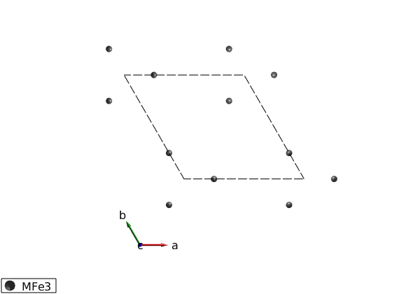
We define only the magnetic atoms in of the crystal that are Fe3+ ions with spin quantum number of 5/2.

banb = spinw;
banb.genlattice('lat_const',[8.539 8.539 5.2414],'angled',[90 90 120],'sym','P 3 2 1');
banb.addatom('label','MFe3','r',[0.24964 0 1/2],'S',5/2,'color','gray');
banb.gencoupling;
plot(banb,'range',[-0.5 1.5;-0.5 1.5;0 0.5])

Chrality

We define three chiral properties of the crystal and magnetic order: * epsilon_T: crystal chirality, in our case we select J3-J5 interactions according to the chirality (J5>J3). * epsilon_Delta: Chirality of the triangular units. * epsilon_H: Sense of rotation of the spin helices along the c-axis (right handed rotation is positive). The three property are related: eT = eD*eH.

eD = -1;
eH = +1;
eT = eD*eH;

Magnetic Hamiltonian

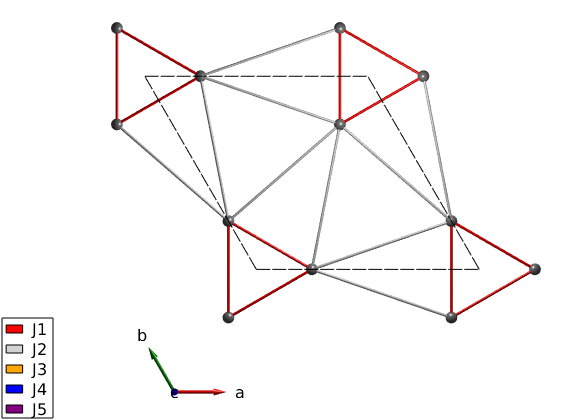
We define the magnetic Hamiltonian depending on the epsilon_T crystal chirality. We neglect the Dzyaloshinskii-Moriya interaction, that can be introduced in a straightforward manner.

J1 = 0.85;
J2 = 0.24;
J3 = 0.053;
J4 = 0.017;
J5 = 0.24;

banb.addmatrix('value',J1,'label','J1','color','red')
banb.addmatrix('value',J2,'label','J2','color','lightgray')
banb.addmatrix('value',J3,'label','J3','color','orange')
banb.addmatrix('value',J4,'label','J4','color','b')
banb.addmatrix('value',J5,'label','J5','color','purple')

banb.addcoupling('mat','J1','bond',1)
banb.addcoupling('mat','J2','bond',3)
banb.addcoupling('mat','J4','bond',2)

switch eT
    case +1
        banb.addcoupling('mat','J3','bond',4)
        banb.addcoupling('mat','J5','bond',5)
    case -1
        banb.addcoupling('mat','J3','bond',5)
        banb.addcoupling('mat','J5','bond',4)
end

plot(banb,'range',[-0.5 1.5;-0.5 1.5;0 0.5],'atomLegend',false)
swplot.zoom(1.3)

Magnetic structure

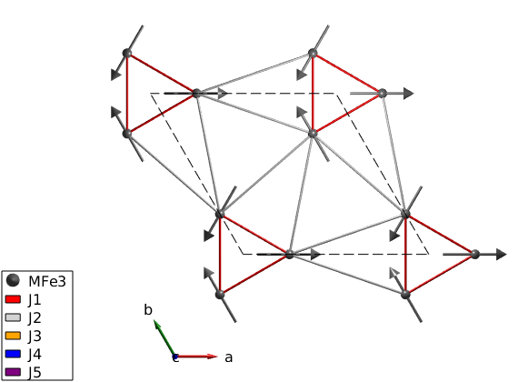
We fix the magnetic structure with the predefined chirality. The magnetic ordering wave vector is k=(0,0,e_H*1/7), the spins are lying in the ab-plane and we use a single cell to describe the structure (default value of nExt = [1 1 1]). We plot the triangular plane magnetic structure.

S0 = [1 -1/2 -1/2;0 eD*sqrt(3)/2 -eD*sqrt(3)/2;0 0 0];
banb.genmagstr('mode','helical','S',S0,'k',[0 0 eH*1/7],'n',[0 0 1])
plot(banb,'range',[-0.5 1.5;-0.5 1.5;0 0.5],'magCentered',true)
swplot.zoom(1.3)
E1 = banb.energy;

% Keep the manual magnetic structure.
Mag0 = banb.mag_str;

Alternatively we optimize the magnetic structure

First we find the propagation vector, then determine the moment directions. We find a slightly lower energy by allowing a tiny deviation from the propagation vector of [0 0 1/7].

banb.optmagk
banb.optmagsteep('nRun',1e4)
banb.genmagstr('mode','rotate','n',[0 0 1])
E2 = banb.energy;
E2-E1

% The vetor normal to the rotation is opposite compared to the manual
% magnetic structure, while the propagation vector is the same. Thus the
% optimized magnetic structure has opposite chirality than the manual
% structure. So we should change the chirality. Instead we restore the
% manual magnetic structure.
banb.mag_str = Mag0;

ans = 

  struct with fields:

       k: [3×1 double]
       E: -5.4522
       F: [3×3 double]
    stat: [1×1 struct]

Warning: Some spins are coupled to themselves in the present magnetic cell! 

ans =

  -1.1400e-06

Spin wave spectrum

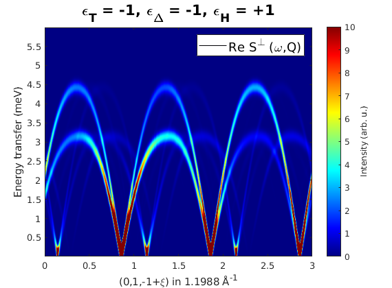
We calculate the spin wave spectrum and compare it to published results. Since the momentum transfer vector Q has opposite sign in SpinW and in the published PRL paper, we change the sign manually here. Also for direct comparison, we calculate the spin-spin correlation function in the coordinate system commonly used for polarised neutron scattering (x||Q, z perpendicular to the scattering plane). To define the scattering plane, we give two reciprocal space vectors in that plane: u=(0,1,0) and v=(0,0,1).

banbSpec = banb.spinwave({[0 -1 1] [0 -1 -2] 500});
banbSpec.hkl  = -banbSpec.hkl;
banbSpec.hklA = -banbSpec.hklA;
banbSpec = sw_neutron(banbSpec,'pol',true,'uv',{[0 1 0] [0 0 1]});

figure
banbSpec = sw_egrid(banbSpec,'component','Sperp','Evect',linspace(0,6,500));
sw_plotspec(banbSpec,'mode','color','dE',0.25,'axLim',[0 10]);
tString = sprintf('\\epsilon_T = %+d, \\epsilon_\\Delta = %+d, \\epsilon_H = %+d',eD,eT,eH);
title(tString,'fontSize',16)
colormap(jet)

Warning: To make the Hamiltonian positive definite, a small omega_tol value was
added to its diagonal! 

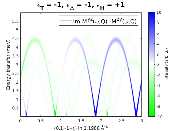
Chiral correlations

We plot the imaginary part of the spin-spin correlation function: Myz-Mzy that are components in the Q coordinate system, this agrees well with Fig. 5 of PRL 106, 207201 (2011).

figure
banbSpec = sw_egrid(banbSpec,'component','Myz-Mzy','Evect',linspace(0,6,500));
sw_plotspec(banbSpec,'mode','color','dE',0.25,'axLim',[-10 10],'imag',true);
tString = sprintf('\\epsilon_T = %+d, \\epsilon_\\Delta = %+d, \\epsilon_H = %+d',eD,eT,eH);
title(tString,'fontSize',16)
colormap(makecolormap([0 1 0],[1 1 1],[0 0 1],81));

Written by
Sandor Toth
16-Jun-2014, 06-Feb-2017

Published with MATLAB® R2018b