Symbolic spin wave dispersion of FM chain
To prepare for symbolic calculation we will need the Matlab Symbolic Toolbox. The symbolic mode should be switched on just after the sw object is created using the sw.symbolic(true) function. The lattice (lattice constants, angles, atomic positions) will still have numerical values. However the spins will be symbolic automatically, see below. The sw.unit_cell.S variable will belong to the 'sym' class, that is defined by the Symbolic Toolbox.
Contents
Define the lattice
FMchain = spinw;
FMchain.symbolic(true)

FMchain.genlattice('lat_const',[3 4 4])
FMchain.addatom('label','A1','r',[0 0 0],'S',1)
disp('Symbolic spin value:')
FMchain.unit_cell.S
FMchain.gencoupling
Warning: The magnetic form factor for A1 is undefined, constant 1 will be used
instead!
Warning: The x-ray scattering form factor for A1+ is undefined, constant 1 will
be used instead! If you don't want to see this message add a line to xrayion.dat
(use the 'edit xrayion.dat' command) for the corresponding ion!
Warning: The neutron scattering length for A1 is undefined, constant 1 will be
used instead!
Symbolic spin value:

ans =

S_1
Magnetic Hamiltonian
When we define the magnetic Hamiltonian, the sw.matrix.mat matrix will contain symbolic values. The values will be the symbolic variable created from the 'label' option and the 'value' matrix. If the input for the 'value' option is symbolic, then it is directly assigned to the sw.matrix.mat field. For the sw.addcoupling(), sw.addaniso(), sw.addg() functions the 'label' value of the matrix has to be used instead of the stored symbolic values. It simplifies the calculation if appropriate assumptions are given for the symbolic variables. In our case, we assume J is positive and use -J for the coupling.
FMchain.addmatrix('label','J1','value',1/2)
disp('Symbolic matrix value from double type input:')
FMchain.matrix.mat

FMchain.addmatrix('label','J1','value',-sym('J','positive'))
disp('Symbolic matrix value from symbolic input:')
FMchain.matrix.mat

FMchain.addcoupling('mat','J1','bond',1)
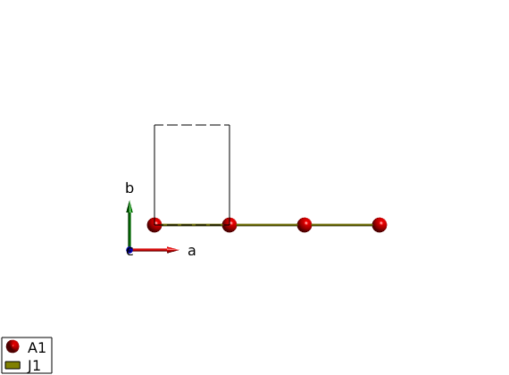
plot(FMchain,'range',[3 0.5 0.5])
Symbolic matrix value from double type input:

ans =

[ J1/2,    0,    0]
[    0, J1/2,    0]
[    0,    0, J1/2]

Symbolic matrix value from symbolic input:

ans =

[ -J,  0,  0]
[  0, -J,  0]
[  0,  0, -J]

Magnetic structure
We can define the magnetic structure as usuall. The normalized symbolic spin components will be created. Beside the magnetic structure can be also created using symbolic input variables, for example incommensurate k-vector, etc.
FMchain.genmagstr('mode','helical','S',[0; 1; 0])
FMchain.magtable.M
plot(FMchain,'range',[3 0.5 0.5],'zoom',1)
ans =

   0
 S_1
   0

Warning: A symbolic magnetic structure can not be plotted.

Ground state energy
The ground state energy can be calculated for symbolic mode as well.
disp('Ground state energy meV/spin:')
FMchain.energy
Ground state energy meV/spin:
Ground state energy (1/spin):
           2
E == -J S_1
Spin wave dispersion
For symbolic mode, only the spin wave dispersion can be calculated calling the sw.spinwave function. It produces the general dispersion withouth any additional input. We note that the final result is not in a nice form, but this is the limitation of the simplify() function of the symbolic engine.
FMspec = FMchain.spinwave();
pretty(FMspec.omega)
Warning: No hkl value was given, spin wave spectrum for general Q (h,k,l) will
be calculated!
/                                        2 \
|  J S_1 exp(-pi h 2i) (exp(pi h 2i) - 1)  |
|                                          |
|                                        2 |
\ -J S_1 exp(-pi h 2i) (exp(pi h 2i) - 1)  /
Plot spin wave spectrum
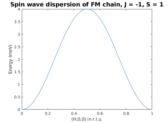
For plotting we need to calculate the spin wave spectrum at given Q point, here along the (H,0,0) direction using the eval() function.
h   = linspace(0,1,501);
J   = 1;
S_1 = 1;
w = real(eval(FMspec.omega(2)));

figure
plot(h,w)
xlabel('(H,0,0) in r.l.u.')
ylabel('Energy (meV)')
title('Spin wave dispersion of FM chain, J = -1, S = 1','fontsize',15)

Written by
Sandor Toth
16-June-2014