Spin wave spectrum of Yb2Ti2O7

This tutorial reproduces the calculated spin wave spectrum of YbLATEX_2PATEXTiLATEX_2PATEXOLATEX_7PATEX with the magnetic Hamiltonian proposed in the following paper: PRX 1 , 021002 (2011).

Create crystal structure
Plot cubic environment of YbLATEX^{3+}PATEX
Create spin Hamiltonian
Plot the magnetic Hamiltonian
Calculate spin wave spectrum

Create crystal structure

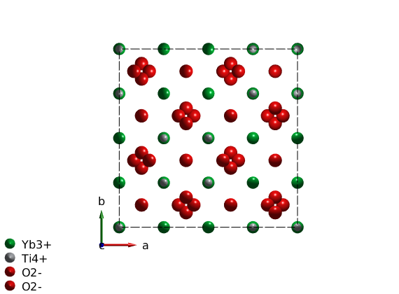
To create the cubic crystal structure of YbLATEX_2PATEXTiLATEX_2PATEXOLATEX_7PATEX, we add a user defined space group with the symmetry generators using the sw_addsym() function. We use the room temperature lattice parameter, however the exact lattice parameter is unimportant for the spin wave calculation as long as we are using lattice units. The spin of the magnetic atoms are automatically created from the ion label that contains the ionic charge after the element label. We also define the non-magnetic atoms for plotting. ALternatively a .cif file of the crystal structure can be imported.

symStr = '-z, y+3/4, x+3/4; z+3/4, -y, x+3/4; z+3/4, y+3/4, -x; y+3/4, x+3/4, -z; x+3/4, -z, y+3/4; -z, x+3/4, y+3/4';

ybti = spinw;
a = 10.0307;
ybti.genlattice('lat_const',[a a a],'angled',[90 90 90],'spgr',symStr,'label','F d -3 m Z')
ybti.addatom('label','Yb3+','r',[1/2 1/2 1/2],'S',1/2)
ybti.addatom('label','Ti4+','r',[0 0 0])
ybti.addatom('label','O2-','r',[0.3318 1/8 1/8])
ybti.addatom('label','O2-','r',[3/8 3/8 3/8])
plot(ybti,'nMesh',3)
swplot.legend('none')

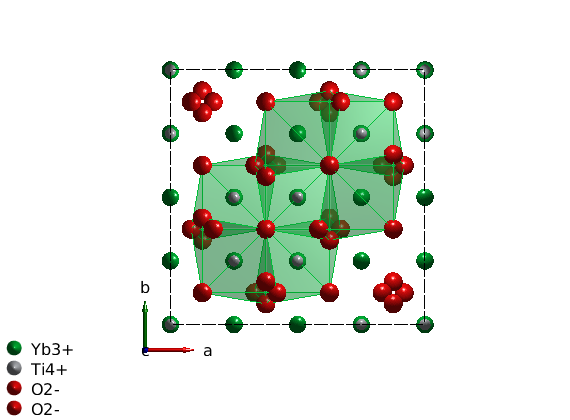
Plot cubic environment of YbLATEX^{3+}PATEX

To the draw oxygen polyhedra around the Yb ions, we use the swplot.plotchem() function, that can draw polyhedra around arbitrary atoms on an existing crystal structure plot. Now we use center atom 'Yb' and polyhedra atoms 'O' for oxygen. Since the oxygen environment of Yb is octahedron, we set the limits to the 8 closes oxygen atom. The same can be achieved within the spinw.plot() function, adding the options below plus a string 'chem', such as 'chemAtom1', 'chemAtom2', 'chemLimit' and 'chemRange' and setting 'chemMode' to 'poly'.

swplot.plotchem('atom1','Yb','atom2','O','limit',8,'range',[0.1 0.9;0.1 0.9;0.1 0.9]);

Create spin Hamiltonian

We can remove the non-magnetic atoms from the spinw object with a single command using the unitcell() function (not to mix with the unit_cell property of the sw object). The unitcell() function can return selected atoms from the list of symmetry inequivalent atoms in the unit cell. In our case the magnetic Yb ions are the first atom.

ybti.unit_cell = ybti.unitcell(1);

% We generate the list of bonds.
ybti.gencoupling

% We create two 3x3 matrix, one for the first neighbor anisotropic exchange
% and one for the anisotropic g-tensor. And assign them appropriately.

ybti.addmatrix('label','J1','value',1)
ybti.addmatrix('label','g0','value',1);

ybti.addcoupling('mat','J1','bond',1)
ybti.addg('g0')

In the paper the anisotropic g-tensor is defined in the local coordinate system of the magnetic ions. Where the LATEXg_zPATEX component is along the local [1 1 1] direction, while the two perpendicular components are LATEXg_{xy}PATEX. In the lattice corrdinate system the g-tensor has the matrix form: [A B B;B A B;B B A]. One can check the eigenvalues of this matrix, that has to match with the published values: LATEXg_{xy}=4.32PATEX and LATEXg_z=1.8PATEX. From the eigenvalue calculation we get: LATEXg_{xy}=A-BPATEX; LATEXg_z = A + 2*BPATEX. We store the calculated g-tensor in the sw object. When calculating the spin wave intensities, the code takes care the rotation of the g-tensor according the symmetry operators for every magnetic ion.

ybti.matrix.mat(:,:,2) =  -0.84*ones(3)+4.32*eye(3);

The SpinW code also enables the calculation of the symmetry allowed exchange matrix elements usign the spinw.getmatrix() function (it also works g-tensor and anisotropy matrix). The allowed matrix elements are defined on the first bond in the ybti.couplingtable(1), thus this is not necessary identical with the bond where the exchange values define in the paper.

ybti.getmatrix('mat','J1');

We assign the exchange values from the paper to the right matrix elements.

J1 = -0.09; J2 = -0.22; J3 = -0.29; J4 = 0.01;
ybti.setmatrix('mat','J1','pref',[J1 J3 J2 -J4]);

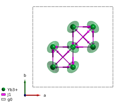
Plot the magnetic Hamiltonian

With the plot() command, we can plot the magnetic bonds of YbLATEX_2PATEXTiLATEX_2PATEXOLATEX_7PATEX. The arrow pointing from an atom to another denotes the direction of the bond, while the thicker arrow at the middle of the bond denotes the direction of the Dzyaloshinskii-Moriya vector. Is is also possible to visualize the g-tensor by setting the 'ionMode' to 'g'.

plot(ybti,'ionMode','g')
swplot.zoom(1.3)
swplot.legend('none')

Calculate spin wave spectrum

We define two different magnetic field direction and field strength in Tesla units same as in the paper and define the list of Q scans.

n = [1 -1 0];
B1 = 5;
B2 = 2;

Q = {};
Q{1} = {[-0.5 -0.5 -0.5] [2 2 2]};
Q{2} = {[1 1 -2] [1 1 1.5]};
Q{3} = {[2 2 -2] [2 2 1.5]};
Q{4} = {[-0.5 -0.5 0] [2.5 2.5 0]};
Q{5} = {[0 0 1] [2.3 2.3 1]};

% To reproduce the simulated spin wave dispersions, we loop over the
% different Q direction. To determine the ground state structure in the
% external field, we use polarised starting state, then using a steepest
% descendent method, we determine the optimum magnetic structure (see
% spinw.optmagsteep() function). For the spin wave spectrum calculation we
% set the 'gtensor' option to true. In this case the code takes care that
% the anisotropic g-tensor is included in the calculated spin wave
% intensity. For the plotting of the spin wave spectrum, a Gaussing with
% FWHM=0.09 meV is convoluted to the spectrum to simulate the finite energy
% resolution.

figure('position',[20 20 1100 500])
for ii = 1:10

    if ii <= 5
        B = B1;
    else
        B = B2;
    end
    % set magnetic field
    ybti.field(n/norm(n)*B);

    if (ii == 1) || (ii==6)
        % create fully polarised magnetic structure along the field direction
        ybti.genmagstr('S',n','mode','helical');
        % find best structure using steepest descendend
        ybti.optmagsteep
    end

    % spin wave spectrum
    ybtiSpec = ybti.spinwave([Q{mod(ii-1,5)+1} {200}],'gtensor',true);
    % neutron scattering cross section
    ybtiSpec = sw_neutron(ybtiSpec);
    % bin the spectrum in energy
    ybtiSpec = sw_egrid(ybtiSpec,'Evect',linspace(0,2,500),'component','Sperp');

    % subplot
    subplot(2,5,ii)
    % colorplot with finite energy resolution of FWHM = 0.09 meV
    sw_plotspec(ybtiSpec,'axLim',[0 0.5],'mode',3,'dE',0.09,'colorbar',false,'legend',false);
    title('')

    caxis([0 60])
    colormap(jet)
end

Tutorial 20