Description

This tutorial fits a spinwave model to simulated powder data.

Define instrument resolution parameters for MARI
Generate data
Initialise the sw_fitpowder class and plot data to inspect initial guess
Fit and inspect the result
Fit 1D cuts

Define instrument resolution parameters for MARI

This is a simplified parameterisation of the resolution of a Time-of-Flight spectrometer which will be used to broaden the simulated data. These parameters will depend on the instrument used - the instrument contact should be able to provide these.

Ei = 20; % meV

% Resolution for MARI with Gd chopper running at 200Hz and Ei=20meV (from PyChop)
eres = @(en) 2.1750e-04*sqrt((Ei-en).^3 .* ( (32.27217*(0.168+0.400*(Ei./(Ei-en)).^1.5)).^2 + (14.53577*(1.168+0.400*(Ei./(Ei-en)).^1.5)).^2) );
% Q-resolution (parameters for MARI)
e2k = @(en) sqrt( en .* (2*1.67492728e-27*1.60217653e-22) )./1.05457168e-34./1e10;
L1 = 11.8;  % Moderator to Sample distance in m
L2 = 4.0;   % Sample to detector distance in m
ws = 0.05;  % Width of sample in m
wm = 0.12;  % Width of moderator in m
wd = 0.025; % Width of detector in m
ki = e2k(Ei);
a1 = ws/L1; % Angular width of sample seen from moderator
a2 = wm/L1; % Angular width of moderator seen from sample
a3 = wd/L2; % Angular width of detector seen from sample
a4 = ws/L2; % Angular width of sample seen from detector
dQ = 2.35 * sqrt( (ki*a1)^2/12 + (ki*a2)^2/12 + (ki*a3)^2/12 + (ki*a4)^2/12 );

Generate data

Simulate a powder spectrum of a triangular AFM with constant background and normally distributed noise. This can also be done using the powder fitting class if an empty data array is passed.

% intialise spinw model
tri = sw_model('triAF',1);
scale = 1000;

% calculate powder spectrum
E = linspace(0,4,80);
Q = linspace(0.1,3,60);
spec = tri.powspec(Q,'Evect',E,'nRand',2e2);
% scale data and add background
spec.swConv= scale*(spec.swConv + 0.1*mean(spec.swConv, 'all'));
% crop to kinematic range of instrument and apply some arbitrary resolution
spec = sw_instrument(spec, 'dQ', dQ, 'dE', eres, 'ThetaMin', 3.5, 'Ei', Ei);
% add noise
e = sqrt(spec.swConv);
spec.swConv = spec.swConv + e.*randn(size(spec.swConv));

% make xye struct containing data
data = struct('x', , ...
              'y', spec.swConv', ...
              'e', e');

Initialise the sw_fitpowder class and plot data to inspect initial guess

To initialise the powder fitting class (sw_fitpowder) object requires a spinw model with a magnetic strucutre and couplings added. Additional arguments are the data (can be xye structs for 2D data a cell array of xye structs for 1D data, or HORACE objects - see sw_fitpowder help for more details), a fit function which alters the matrices on the spinw object and a vector of initial guesses for the fit parameters.

Optinally a background strategy can be specified as a 5th positional argument ("planar" background in energy transfer and Q or "independent" background for each 1D cut (1D only)).

The class will call other spinw algorithms such as powspec and sw_instrument. The parameters used in these calls can be set by the user by modifying structs as shown below.

Data can be cropped in Q and energy transfer - for example it is advisible not to include the low-energy transfer region close to the elastic line (relative to the resolution).

fit_func =  @(obj, p) matparser(obj, 'param', p, 'mat', {'J_1'}, 'init', true);
J1 = 0.85;

fitpow = sw_fitpowder(tri, data,  fit_func, [J1]);
fitpow.set_caching(true); % will store last calculated spectra

% set parameters passed to powspec
fitpow.powspec_args.dE = eres; % emergy resolution
fitpow.powspec_args.fastmode = true;
fitpow.powspec_args.neutron_output = true;
fitpow.powspec_args.nRand = 2e2; % low for speed (typically want > 1e3)
fitpow.powspec_args.hermit = true;
% set parameters passsed to sw_instrument
fitpow.sw_instrument_args = struct('dQ', dQ, 'ThetaMin', 3.5, 'Ei', Ei);

% crop data
fitpow.crop_energy_range(1.5*eres(0), inf); % typically want to avoid elastic line
fitpow.crop_q_range(0.25, 3);
fitpow.powspec_args.dE = eres;
fitpow.powspec_args.fastmode = true;
fitpow.powspec_args.neutron_output = true;

% estimate background and scale factor
fitpow.estimate_constant_background();
fitpow.estimate_scale_factor();


% plot data to inspect - any arguments after parameters are passed to
% contour plot (which shows the result the calculated intensity)
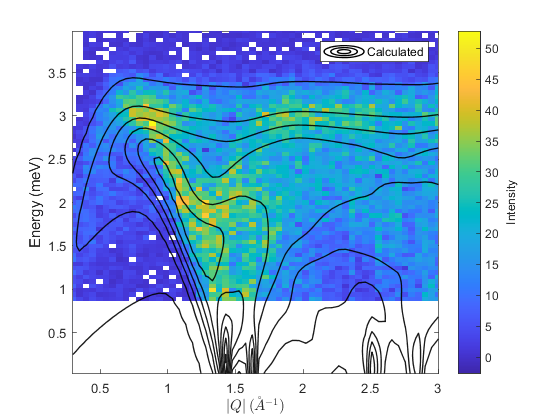
fitpow.plot_result(fitpow.params, 'EdgeAlpha', 0.9, 'LineWidth', 1 ,'EdgeColor', 'k');

Fit and inspect the result

It can be desirable to set bounds on fit parameters and fix some parameters initially to get a reasonable fit with as few degrees of freedom as possible. For example one might assume the background is constant in an initial fit.

The cost function minimised in the fit can be chi-squared ("chisq") or the unweighted sum of the squared residuals ("Rsq"). Also the minimiser can be set to any callable as long as it shares the API of the ndbase minimisers. Typically users would be recommended ndbase.lm or ndbase.simplex.

% set cost function and minimser
fitpow.cost_function = "Rsq";  % "Rsq" or "chisq"
fitpow.optimizer = @ndbase.simplex; % or e.g. ndbase.simplex

% Fix background parameters (planar background of form
% default background is planar with parameters:
% [slope_energy, slope_modQ,  intercept]
fitpow.fix_bg_parameters(1:2); % fix slopes to initial value (0)
fitpow.set_bg_parameter_bounds(3, 0.0, []) % Set lb of constant bg = 0
% fit background
fitpow.fit_background();
fitpow.fix_bg_parameters(3); % fix fitted constant bg

% set bounds on first (and only in this case) model parameter
fitpow.set_model_parameter_bounds(1, 0, []) % Force J_1 to be AFM

[pfit, cost_val, stat] = fitpow.fit();

% plot 2D colorfill
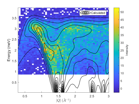
fitpow.plot_result(pfit, 10,  'EdgeAlpha', 0.9, 'LineWidth', 1 ,'EdgeColor', 'k')

% make 1D plots
qcens = [0.8:0.4:1.6];
dq = 0.05;
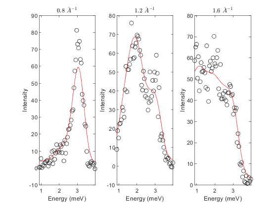
fitpow.plot_1d_cuts_of_2d_data(qcens-dq, qcens+dq, pfit)

Fit 1D cuts

As discussed the sw_fitpowder class can be initialised with a cell array of xye structs correpsonding to 1D cuts at constant Q. Alternatively, having loaded in 2D data the sw_fitpowder class has a convenient method to take 1D cuts and replace the data.

To evaluate the cost function for 1D cuts, the class averages the model over nQ points. Depending on the size of the 2D data and the value of nQ it can be much quicker to fit 1D cuts.

The background for 1D cuts can be handled in two ways:

- A planar background as in the 2D case

- A linear background in energy transfer that's independent for each cut.

The background parameters and bounds are reset if the background strategy is changed to independent.

% set nQ before replacing data (reduced from default, 10, for speed)
fitpow.nQ = 5;
% change background strategyto independent (planar is default)
fitpow.replace_2D_data_with_1D_cuts(qcens-dq, qcens+dq, "independent");

% independent linear background for all cuts with parameters:
% [slope_energy,  intercept]
fitpow.fix_bg_parameters(1); % fix slopes to initial value (0) for all cuts
% e.g. fitpow.fix_bg_parameters(1, 2) would fix the bg slope of the second cut
fitpow.set_bg_parameter_bounds(2, 0.0, []) % Set lb of constant bg = 0
% fit background
fitpow.estimate_constant_background();
fitpow.fit_background();
fitpow.fix_bg_parameters(2); % fix fitted constant bg

[pfit, cost_val, stat]  = fitpow.fit();

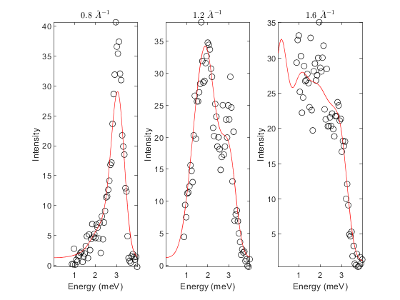
fitpow.plot_result(pfit)

Warning: Clearing 2D data previously added. 
Warning: Overwriting background parmaweters with 0. 
Warning: Background strategy changed - background parameters and bounds
will be cleared.

Tutorial 39