Square-lattice antiferromagnet#

This tutorial mirrors MATLAB spinW Tutorial 4

In this tutorial we will show how to calculate the magnon spectrum for a square lattice antiferromagnet, and in particular for the case of La\(_2\)CuO\(_4\) (Coldea et al., Phys. Rev. Lett. 86 5377 (2001).

As previously, we import pyspinw, and this time we also import matplotlib.

from pyspinw import *
import matplotlib.pyplot as plt

A J1-J2 antiferromagnet on a square lattice#

First we examine the case of a square lattice with a strong antiferromagnetic first neighbour and weak ferromagnetic second neighbour Heisenberg interactions with the following parameters:

ordering wave vector \(\mathbf{k} = (\frac{1}{2} \frac{1}{2} 0)\)
spins in the \(a\)-\(b\) plane (the spins can have an arbitrary phase so we fix this by defining them to be parallel/anti-parallel to \(a\)).

unit_cell = UnitCell(3, 3, 9)
sites = [Site(0, 0, 0, 1, 0, 0, name="X")]
k = CommensuratePropagationVector(0.5, 0.5, 0)
struc = Structure(sites, unit_cell, supercell=SummationSupercell(propagation_vectors=[k]))

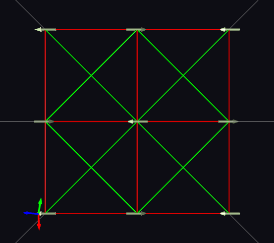
Next we define the exchange interaction with a large positive (AFM) nearest neighbour \(J_1\) and a small negative (FM) next-nearest neighbour \(J_2\) and form the Hamiltonian and plot it

exchanges = generate_exchanges(struc, bond=1, j=1, color=[1,0,0]) + \
            generate_exchanges(struc, bond=2, j=-0.1, color=[0,1,0])
hamiltonian = Hamiltonian(struc, exchanges)
hamiltonian.print_summary()

view(hamiltonian)

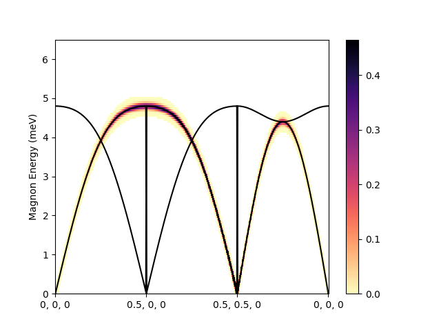
Now we calculate the magnon spectrum along the main in-plane wavevectors

path = Path([[0,0,0], [0.5,0,0], [0.5,0.5,0], [0,0,0]], n_points_per_segment=201)
fig = hamiltonian.spaghetti_plot(path, show=False)
fig.axes[0].set_ylim(0, 6.5)

plt.show()

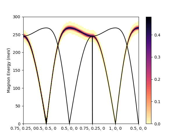
The case of La\(_2\)CuO\(_4\)#

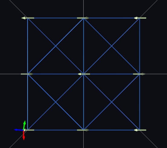
We now reproduce the model of La\(_2\)CuO\(_4\), the parent of one of the family of high temperature cuprate superconductors, from Coldea et al., Phys. Rev. Lett. 86 5377 (2001), which has three nearest-neighbour interactions

j1 = generate_exchanges(struc, bond=1, exchange_type=HeisenbergExchange, j=59.65)
j2 = generate_exchanges(struc, bond=2, exchange_type=HeisenbergExchange, j=-3.75)
j3 = generate_exchanges(struc, bond=3, exchange_type=HeisenbergExchange, j=1)
hamiltonian = Hamiltonian(struc, j1 + j2 + j3)
hamiltonian.print_summary()

view(hamiltonian)

This time we use a slightly different path to emphasise the effect of the third neighbour interaction in the \(X - P, (\frac{1}{2}00)-(\frac{3}{4}\frac{1}{4}0)\) direction.

path = Path([[3/4, 1/4, 0], [1/2, 1/2, 0], [1/2, 0, 0], [3/4, 1/4, 0], [1, 0, 0], [1/2, 0, 0]], n_points_per_segment=201)
fig = hamiltonian.spaghetti_plot(path, show=False)
fig.axes[0].set_ylim(0, 300)

plt.show()