
Tutorial 5#
Ferromagnetic first neighbor Kagome lattice#
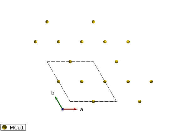
We define the kagome lattice using the “P -3” space group (Nr. 147), using the 3 fold symmetry, we need to define only one magnetic atom. In this space group all fisrt neighbor couplings will be equivalent (related by symmetry). Symmetry equivalent positions of the magnetic atoms are automatically generated by the spinw.matom method. The magnetic atoms are Cu+ with S=1 spin.
Define the lattice#
FMkagome = spinw;
FMkagome.genlattice('lat_const',[6 6 5],'angled',[90 90 120],'spgr','P -3')
FMkagome.addatom('r', [1/2 0 0], 'S', 1, 'label','MCu1','color','r')
disp('Magnetic atom positions:')
FMkagome.table('matom')
plot(FMkagome,'range',[2 2 1],'atomColor','gold')
Magnetic atom positions:

ans =

  3x4 table

    matom     idx    S           pos
    ______    ___    _    _________________

    'MCu1'     1     1    0.5      0      0
    'MCu1'     2     1      0    0.5      0
    'MCu1'     3     1    0.5    0.5      0
Create FM bonds#
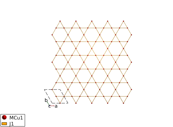
The first neighbor bonds will be ferromagnetic, J = -1 meV. The spinw.gencoupling will use the space group operators to identify equivalent couplings, if two bonds have the same length but not symmetry related, then they will be identified as different bonds. The ‘maxDistance’ option of the spinw.gencoupling method will be ensure that all bonds are generated up to the given distance in Angstrom.
FMkagome.gencoupling('maxDistance',4)
disp('Bonds (length in Angstrom):')
FMkagome.table('bond',[])

FMkagome.addmatrix('label','J1','value',-1,'color','orange');
FMkagome.addcoupling('mat','J1','bond',1);

% Plot a nice rectangular cutout of the kagome lattice
plot(FMkagome,'range',[31 32 2],'unit','xyz','cellMode','single')
Bonds (length in Angstrom):

ans =

  6x10 table

    idx    subidx          dl                   dr             length    matom1    idx1    matom2    idx2        matrix
    ___    ______    ______________    ____________________    ______    ______    ____    ______    ____    ______________

     1       1        0     1     0       0     0.5       0      3       'MCu1'     3      'MCu1'     1      ''    ''    ''
     1       2        0    -1     0    -0.5    -0.5       0      3       'MCu1'     1      'MCu1'     2      ''    ''    ''
     1       3        0     0     0     0.5       0       0      3       'MCu1'     2      'MCu1'     3      ''    ''    ''
     1       4        0     0     0       0    -0.5       0      3       'MCu1'     3      'MCu1'     1      ''    ''    ''
     1       5        1     0     0     0.5     0.5       0      3       'MCu1'     1      'MCu1'     2      ''    ''    ''
     1       6       -1     0     0    -0.5       0       0      3       'MCu1'     2      'MCu1'     3      ''    ''    ''
FM magnetic structure#
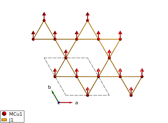
All spins are paralle, pointing along the y-axis (perpendicular to ac plane). We use the “helical” mode of the sw.gencoupling() function, even though the structure is not helical. However in this mode all missing spins will be automatically created using the k-vector and normal vector and assuming helical magnetic structure. Thus if we give k = (0 0 0) and only the direction of the first spin in the unit cell, the code will create all other spin parallel to the first.
FMkagome.genmagstr('mode','helical','k',[0 0 0],'n',[0 1 0],'S',[0 1 0]')
disp('Magnetic structure:')
FMkagome.table('mag')
FMkagome.energy
plot(FMkagome,'range',[2 2 1])
Magnetic structure:

ans =

  3x7 table

    num    matom     idx    S     realFhat             pos              kvect
    ___    ______    ___    _    ___________    _________________    ___________

     1     'MCu1'     1     1    0    1    0    0.5      0      0    0    0    0
     2     'MCu1'     2     1    0    1    0      0    0.5      0    0    0    0
     3     'MCu1'     3     1    0    1    0    0.5    0.5      0    0    0    0

Ground state energy: -2.000 meV/spin.
Spin wave dispersion#
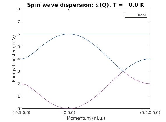
We calculate the spin wave dispersion. There are three modes, equal to the number of magnetic atom in the magnetic unit cell, denoted by different colors. At the zone center, the dispersion of the goldstone mode is parabolic, due to the FM interactions.
fmkSpec = FMkagome.spinwave({[-1/2 0 0] [0 0 0] [1/2 1/2 0] 100},'hermit',false);
fmkSpec = sw_neutron(fmkSpec);
fmkSpec = sw_egrid(fmkSpec, 'Evect',linspace(0,6.5,100),'component','Sperp');
figure
sw_plotspec(fmkSpec,'mode',1,'colorbar',false,'axLim',[0 8])
Powder spectrum#
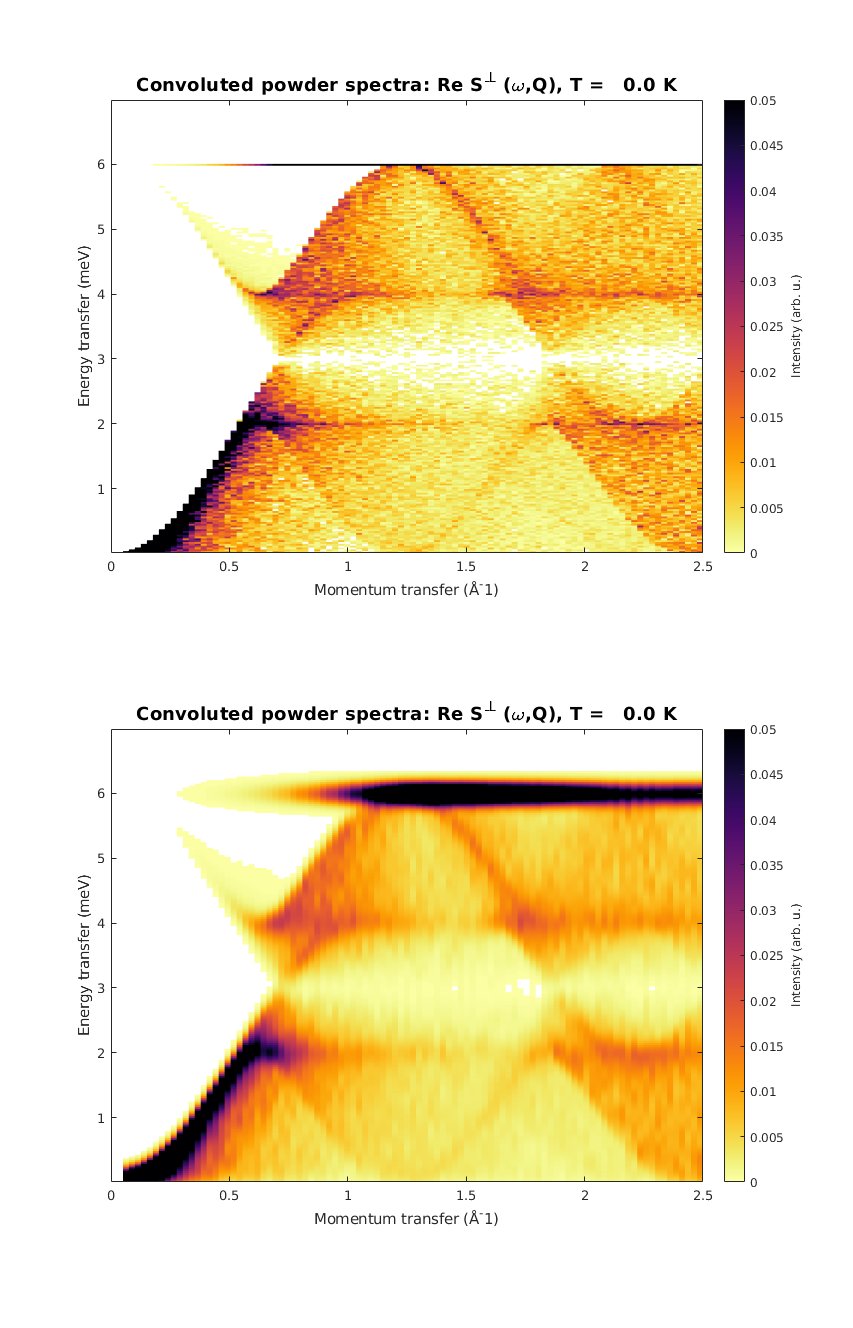
We plot the powder spectrum two different ways. First as calculated (to show the extremely sharp Van Hoove singularity at the top of the dispersion), secondly convolute with a Gaussian along energy.
fmkPow = FMkagome.powspec(linspace(0,2.5,100),'Evect',linspace(0,7,250),'nRand',1000,'hermit',false);
figure
subplot(2,1,1)
sw_plotspec(fmkPow,'colorbar',true,'axLim',[0 0.05])
subplot(2,1,2)
sw_plotspec(fmkPow,'colorbar',true,'axLim',[0 0.05],'dE',0.25,'norm',true)
swplot.subfigure(1,3,1)
Written by
Bjorn Fak & Sandor Toth
06-Jun-2014, 06-Feb-2017
Published with MATLAB® R2018b