
Tutorial 6#
Ferromagnetic kagome lattice#
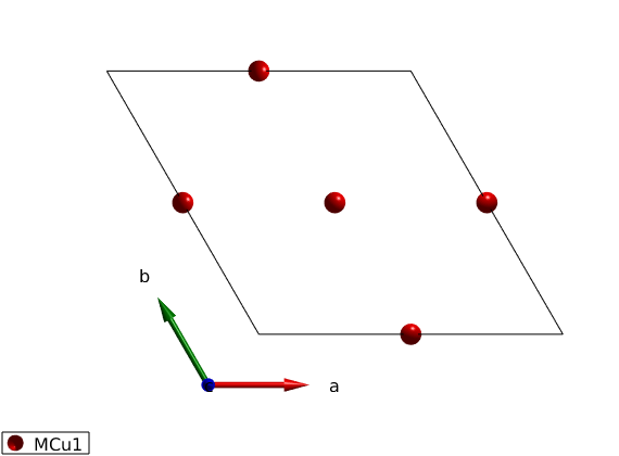
We create the kagome lattice with up to 4th neighbor interactions. The symmetry related atoms are denoted by MCu1(i)_j, where i is the index of independent atomic positions, j is the index of the generated atomic positions of the i-th independent position.
Define the lattice#
kagome4 = spinw;
kagome4.genlattice('lat_const',[6 6 8],'angled',[90 90 120],'spgr','P -3');
kagome4.addatom('r', [1/2 0 0],'S', 1,'label','MCu1','color','r');
disp('Atomic positions:')
kagome4.table('atom')
plot(kagome4)
swplot.zoom(1.5)
Atomic positions:

ans =

  3x4 table

    matom     idx    S           pos
    ______    ___    _    _________________

    'MCu1'     1     1    0.5      0      0
    'MCu1'     2     1      0    0.5      0
    'MCu1'     3     1    0.5    0.5      0
Define Hamiltonian#
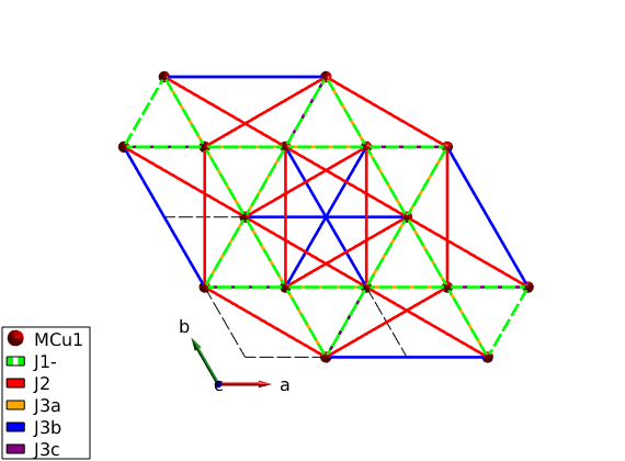
We add couplings up to 4th neighbor interactions. If the generation of the bond tables would depend on distance, J3a, J3b and J3c would be equivalent. However using the ‘P -3’ space group the three type of bonds are inequivalent, as physically expected in real systems (J3a goes through an intermediate magnetic atom, while the other two bonds are not).
kagome4.gencoupling('maxDistance',7);
disp('Bonds:')
kagome4.table('bond',[])

kagome4.addmatrix('label','J1-','value',-1.00,'color','g')
kagome4.addmatrix('label','J2','value', 0.10,'color','r')
kagome4.addmatrix('label','J3a','value', 0.00,'color','orange')
kagome4.addmatrix('label','J3b','value', 0.17,'color','b')
kagome4.addmatrix('label','J3c','value', 0.00,'color','purple')

kagome4.addcoupling('mat','J1-','bond',1);
kagome4.addcoupling('mat','J2','bond',2);
kagome4.addcoupling('mat','J3a','bond',3);
kagome4.addcoupling('mat','J3b','bond',4);
kagome4.addcoupling('mat','J3c','bond',5);

% The first neighbor bonds will be shown as dashed lines. This is automatic
% when the matrix labels ends with a minus sign.
plot(kagome4,'range',[2 2 1],'bondMode','line','bondLineWidth0',2)
Bonds:

ans =

  21x10 table

    idx    subidx          dl                   dr             length    matom1    idx1    matom2    idx2        matrix
    ___    ______    ______________    ____________________    ______    ______    ____    ______    ____    ______________

     1       1        0     1     0       0     0.5       0        3     'MCu1'     3      'MCu1'     1      ''    ''    ''
     1       2        0    -1     0    -0.5    -0.5       0        3     'MCu1'     1      'MCu1'     2      ''    ''    ''
     1       3        0     0     0     0.5       0       0        3     'MCu1'     2      'MCu1'     3      ''    ''    ''
     1       4        0     0     0       0    -0.5       0        3     'MCu1'     3      'MCu1'     1      ''    ''    ''
     1       5        1     0     0     0.5     0.5       0        3     'MCu1'     1      'MCu1'     2      ''    ''    ''
     1       6       -1     0     0    -0.5       0       0        3     'MCu1'     2      'MCu1'     3      ''    ''    ''
     2       1        1    -1     0     0.5    -0.5       0    5.196     'MCu1'     1      'MCu1'     2      ''    ''    ''
     2       2        0     1     0     0.5       1       0    5.196     'MCu1'     2      'MCu1'     3      ''    ''    ''
     2       3       -1     0     0      -1    -0.5       0    5.196     'MCu1'     3      'MCu1'     1      ''    ''    ''
     2       4        0     0     0    -0.5     0.5       0    5.196     'MCu1'     1      'MCu1'     2      ''    ''    ''
     2       5       -1    -1     0    -0.5      -1       0    5.196     'MCu1'     2      'MCu1'     3      ''    ''    ''
     2       6        1     1     0       1     0.5       0    5.196     'MCu1'     3      'MCu1'     1      ''    ''    ''
     3       1        0     1     0       0       1       0        6     'MCu1'     1      'MCu1'     1      ''    ''    ''
     3       2       -1    -1     0      -1      -1       0        6     'MCu1'     2      'MCu1'     2      ''    ''    ''
     3       3        1     0     0       1       0       0        6     'MCu1'     3      'MCu1'     3      ''    ''    ''
     4       1        0     1     0       0       1       0        6     'MCu1'     2      'MCu1'     2      ''    ''    ''
     4       2       -1    -1     0      -1      -1       0        6     'MCu1'     3      'MCu1'     3      ''    ''    ''
     4       3        1     0     0       1       0       0        6     'MCu1'     1      'MCu1'     1      ''    ''    ''
     5       1        0     1     0       0       1       0        6     'MCu1'     3      'MCu1'     3      ''    ''    ''
     5       2       -1    -1     0      -1      -1       0        6     'MCu1'     1      'MCu1'     1      ''    ''    ''
     5       3        1     0     0       1       0       0        6     'MCu1'     2      'MCu1'     2      ''    ''    ''
Magnetic structure#
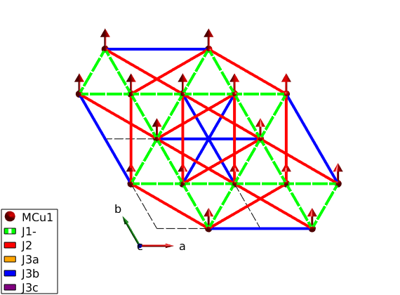
For strong FM 1str neighbour and weak further neighbor interaction the ground state is ferromagnetic.
kagome4.genmagstr('mode','helical','k',[0 0 0],'n',[0 1 0],'S',[0 1 0]');
disp('Magnetic structure:')
kagome4.table('mag')
kagome4.energy
plot(kagome4,'range',[2 2 1],'bondMode','line','bondLineWidth0',3,...
    'bondZero',false)
Magnetic structure:

ans =

  3x7 table

    num    matom     idx    S     realFhat             pos              kvect
    ___    ______    ___    _    ___________    _________________    ___________

     1     'MCu1'     1     1    0    1    0    0.5      0      0    0    0    0
     2     'MCu1'     2     1    0    1    0      0    0.5      0    0    0    0
     3     'MCu1'     3     1    0    1    0    0.5    0.5      0    0    0    0

Ground state energy: -1.630 meV/spin.
Spin wave dispersion#
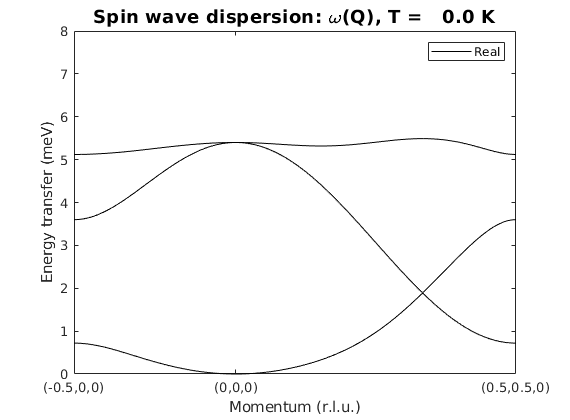
kag4Spec = kagome4.spinwave({[-1/2 0 0] [0 0 0] [1/2 1/2 0] 200});
kag4Spec = sw_neutron(kag4Spec);
kag4Spec = sw_egrid(kag4Spec,'Evect',linspace(0,6.5,100)) ;
figure
sw_plotspec(kag4Spec,'mode',1,'axLim',[0 8],'colorbar',false,'colormap',[0 0 0])
Warning: To make the Hamiltonian positive definite, a small omega_tol value was
added to its diagonal!
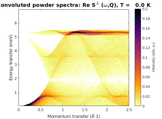
Powder averaged spectrum#
kag4Pow = kagome4.powspec(linspace(0,2.5,100),'Evect',linspace(0,7,250),...
    'nRand',1e3,'hermit',false);
figure
sw_plotspec(kag4Pow,'axLim',[0 0.2],'colorbar',true)
Written by
Bjorn Fak & Sandor Toth
06-Jun-2014, 06-Feb-2017
Published with MATLAB® R2018b